The Tax Agency obtains salary information from the annual information return on withholdings from employment and economic activity income (known as Form 190). The information is comprehensive (all employers are required to submit it) and individual (its data is incorporated into the tax records of each taxpayer's income tax return), making it the best possible source for studying the labor market and wages.

In this regard, previous posts in this newsletter have already discussed how these data are used and how they are integrated into other statistics ( Employment and wages in the Tax Agency statistics ), and the advantages provided by the detail in the information ( Where can I see the minimum wage in tax statistics? ).

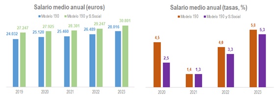
Virtually the only limitation facing the information in Form 190 is the measurement of employment. The model includes all the people who have received wages, but not the length of time they have been receiving those wages. This determines the form of the salary distribution that can be deduced from the data (it can be found in the file Salary distribution ), in which a strong accumulation can be seen in the first sections due to the existence of work periods of less than a year and, above all, the estimate of the average salary. In order to correct this last problem, in statistics Labor market and pensions in tax sources the Full year salary module was introduced since the 2019 publication, which, combined with Social Security data at the individual level, obtains an average salary corrected for working time. The following graphs show the difference in level and rate of change between the usual approach using only Form 190 data and the one corrected using Social Security working time information.

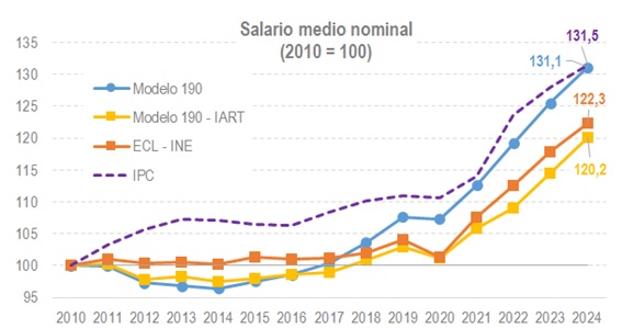
The problem is that this fix has only been available since 2019. As a solution to have a longer series, Table 2.2 of the Annual Tax Collection Report (IART) makes a similar, albeit aggregated, approximation. A level of salaried employment is estimated, based primarily on Social Security affiliation figures, which allows for the average employment for the year to be taken into account, rather than the total number of people who have entered the labor market in a given year, as is the case with Model 190. The result is shown in the following graph.

The graph compares the evolution of the average salary obtained directly from Form 190 and the version of the average salary included in the IART, and is accompanied by the estimate of the average salary published by the INE (Labor Cost Survey, ECL) and the evolution of consumer prices (CPI). As seen in the first graph, the difference between the two versions of Model 190 is significant, especially when compared to price trends. One estimate shows the purchasing power of wages is practically the same as in 2020, while the other, as with the INE data, shows a considerable loss in purchasing power.

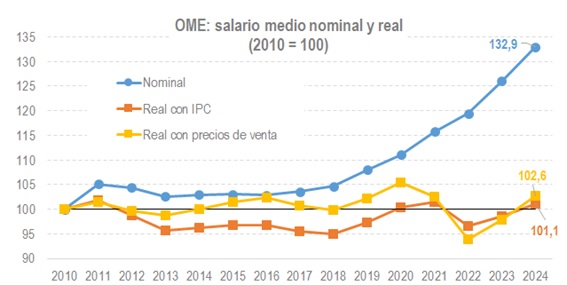
This approach has the limitation that it is performed at the aggregate level. It could be disaggregated by activities or any other variable. However, there is the difficulty of fitting series from different sources without being certain that the classifications are the same; In the case of companies, without knowing whether each of the companies is in the same activity in the two data sources used. Without this certainty, when disaggregating, it is preferable to use information from a single source. This is what is done in the Business Margins Observatory (OME) in which employment is measured by the annual average of the salary recipients declared in the 111 form of employment withholdings. This data also allows for the correlation of salaries with the sales prices offered in the same OME as complementary information. This gives additional perspective: Dividing the average wage by the selling prices results in an indicator of the cost of labor in real terms for the company, distinct from the indicator of the purchasing power of wages, which is the one obtained by dividing by the CPI. The final graph shows that exercise.